frogs <- readr::read_csv('https://raw.githubusercontent.com/rfordatascience/tidytuesday/master/data/2022/2022-08-02/frogs.csv')Overview
This #TidyTuesday week 31 is all about Oregon Spotted a frog: Rana Pretiosa.
Load the {tidyverse} and the data from: #TidyTuesday GitHub repo

Or, as I made a package of these data, the dataset can be installed via:
# install.packages("remotes")
remotes::install_github("fgazzelloni/oregonfrogs")
And then:
library(oregonfrogs)
data(package = 'oregonfrogs')
More about Oregon Frogs and spatial modeling is in this R-Ladies DC talk:
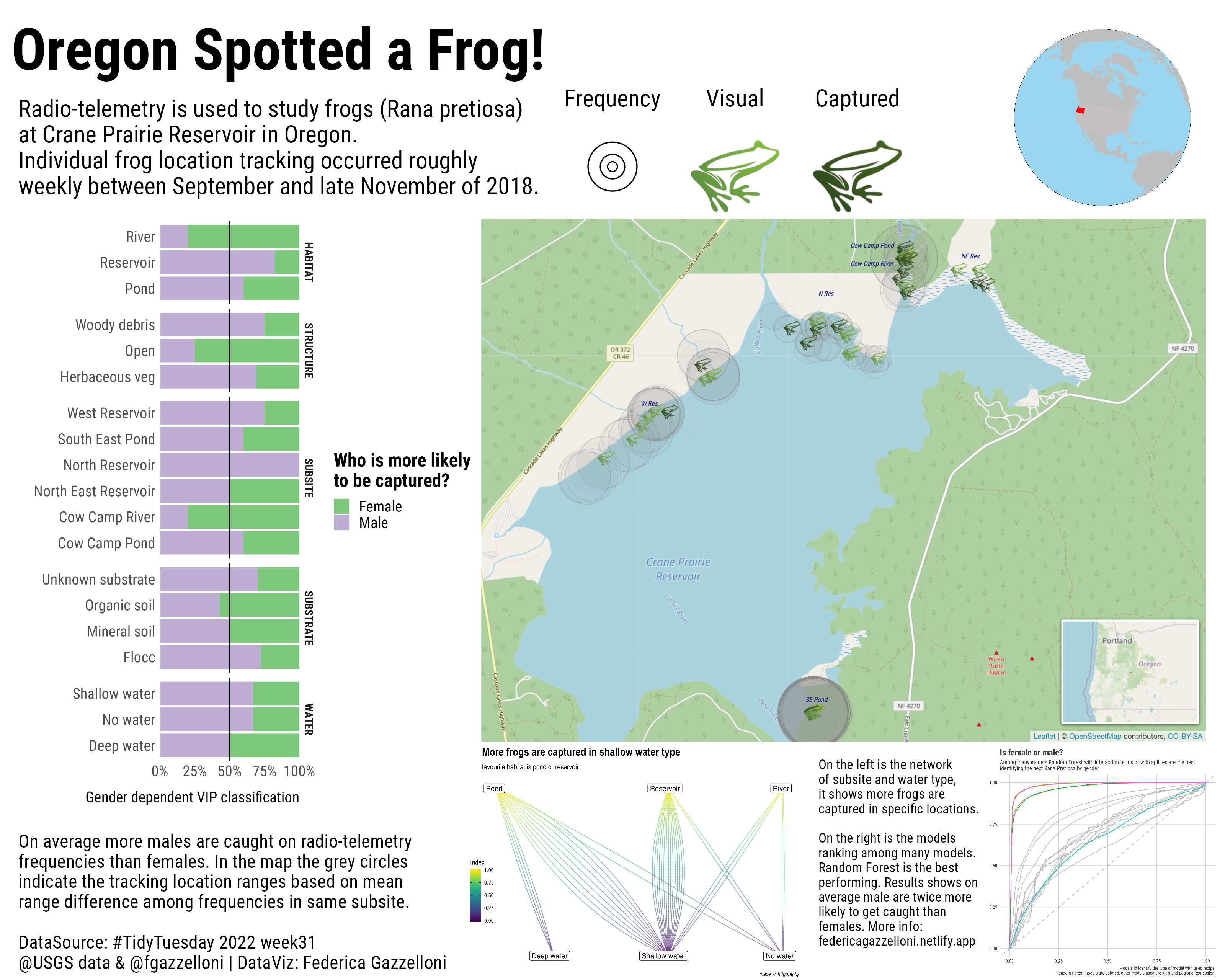
This is the final code for assembling all plots saved in the container images folder using {cowplot} package. In addition, some annotations and grobs are included.
All separate scripts are selfcontainers:
g <- grid::circleGrob(gp = grid::gpar(fill = NA,color="gray"))library(cowplot)
ggdraw() +
draw_label("Oregon Spotted a Frog!",
x=0.227,y=0.95,size=34,
fontface = "bold",
fontfamily = "Roboto Condensed") +
draw_label(label="Captured",x=0.7,y=0.9,fontfamily = "Roboto Condensed") +
draw_label(label="Visual",x=0.6,y=0.9,fontfamily = "Roboto Condensed") +
draw_label(label="Frequency",x=0.5,y=0.9,fontfamily = "Roboto Condensed") +
draw_label(label="Radio-telemetry is used to study frogs (Rana pretiosa)\nat Crane Prairie Reservoir in Oregon.\nIndividual frog location tracking occurred roughly\nweekly between September and late November of 2018.",
fontfamily = "Roboto Condensed",
x=0.015,y=0.85,hjust=0) +
draw_label(label="On average more males are caught on radio-telemetry\nfrequencies than females. In the map the grey circles\nindicate the tracking location ranges based on mean\nrange difference among frequencies in same subsite. \n\nDataSource: #TidyTuesday 2022 week31\n@USGS data & @fgazzelloni | DataViz: Federica Gazzelloni",
fontfamily = "Roboto Condensed",
x=0.015,y=0.08,hjust=0,size=11) +
draw_label(label="On the left is the network\nof subsite and water type,\nit shows more frogs are\ncaptured in specific locations.\n\nOn the right is the models\nranking among many models.\nRandom Forest is the best\nperforming. Results shows on\naverage male are twice more\nlikely to get caught than\nfemales. More info:\nfedericagazzelloni.netlify.app",
fontfamily = "Roboto Condensed",
x=0.668,y=0.13,hjust=0,size=8) +
draw_image("container/images/globe.png",
scale=0.18,
x=0.4,y=0.38)+
draw_image("container/images/network_plot.png",
scale=0.29,
x=0.022,y=-0.38)+
draw_image("container/images/roc_plot.png",
scale=0.245,
x=0.4,y=-0.38)+
draw_image("container/images/lake_map.png",
scale=0.7,
x=0.14,y=0.01) +
draw_image("container/images/vip_plot.png",
scale=0.62,
x=-0.3,y=-0.03)+
draw_image("container/images/frog_logo_visual.png",
scale=0.2,
x=0.1, y=0.32) +
draw_image("container/images/frog_logo_captured.png",
scale=0.2,
x=0.2, y=0.32) +
draw_grob(g, scale = 0.05,x = 0,y = 0.33)+
draw_grob(g, scale = 0.025,x = 0,y = 0.33)+
draw_grob(g, scale = 0.01,x = 0,y = 0.33)# ggsave("w31_frogs.png",
# width=10,
# height = 8,
# dpi=320,
# bg = "white")