How a Model Learns in Epidemiology

A blended teaching workflow combining the mechanics of learning with a real WNV prediction problem

Workshop notebook

Perspectives:

1. a conceptual explanation of how machine learning models learn;
2. a realistic epidemiology workflow for predicting West Nile virus (WNV) activity.

The goal is to understand both the mathematical idea of learning and the practical pipeline used in applied work.

Slide presentation

Open the 12-slide presentation Download the editable PowerPoint

The slide deck introduces the broader multi-model workflow. The model-performance and variable-importance values shown in the deck are illustrative. The executable notebook below contains the observed results.

By the end, we should be able to answer four questions:

1. What is the model?
2. What is the loss?
3. What is the optimisation procedure?
4. What is learned?

The central message is:

Learning means using data to determine a model’s parameters or structure. Optimisation is the procedure used to find useful values or structures according to an objective.

---

1. Model, loss, optimisation, and learning

These terms are connected, but they are not interchangeable.

Concept	Question	Example
Model	How are inputs turned into predictions?	\(\hat y = wx + b\)
Loss	How wrong are the predictions?	Mean squared error
Optimisation	How do we search for a better model?	Gradient descent
Learning	What changes because of the data?	Values of \(w\) and \(b\)

The learning cycle is:

training data
     |
     v
make predictions with the current model
     |
     v
calculate the loss
     |
     v
use an optimisation rule to update the model
     |
     +-------------------- repeat for another epoch

Optimisation is therefore not an extra step after learning. In many models, it is the mechanism through which learning happens.

---

2. A small linear-regression example

To make learning concrete, we begin with a tiny regression example.

library(ggplot2)

theme_set(theme_minimal(base_size = 13))

training_data <- data.frame(
  x = 1:8,
  y = c(2.9, 3.4, 4.5, 5.0, 6.3, 6.7, 7.8, 8.1)
)

training_data

  x   y
1 1 2.9
2 2 3.4
3 3 4.5
4 4 5.0
5 5 6.3
6 6 6.7
7 7 7.8
8 8 8.1

The model is:

\[ \hat y_i = wx_i + b, \]

where:

• \(w\) is the slope;
• \(b\) is the intercept;
• \(\hat y_i\) is the prediction for observation \(i\).

At the start, both parameters are set to zero.

w <- 0
b <- 0

training_data$initial_prediction <- w * training_data$x + b
training_data

  x   y initial_prediction
1 1 2.9                  0
2 2 3.4                  0
3 3 4.5                  0
4 4 5.0                  0
5 5 6.3                  0
6 6 6.7                  0
7 7 7.8                  0
8 8 8.1                  0

---

3. The loss function

We need a way to measure the gap between the observed values and the predictions. We use mean squared error:

\[ \operatorname{MSE}(w,b) = \frac{1}{n}\sum_{i=1}^{n}\left(\hat y_i-y_i\right)^2. \]

mse <- function(observed, predicted) {
  mean((predicted - observed)^2)
}

initial_loss <- mse(
  observed = training_data$y,
  predicted = training_data$initial_prediction
)

initial_loss

[1] 34.53125

A loss value tells us how well the current parameters fit the training data. It does not update the parameters by itself.

---

4. Batch gradient descent from scratch

Example from the article: ml-in-epidemiology-article

Gradient descent asks: in which direction should each parameter move to reduce the loss?

For MSE, the gradients are:

\[ \frac{\partial \operatorname{MSE}}{\partial w} = \frac{2}{n}\sum_{i=1}^{n}(\hat y_i-y_i)x_i \]

and

\[ \frac{\partial \operatorname{MSE}}{\partial b} = \frac{2}{n}\sum_{i=1}^{n}(\hat y_i-y_i). \]

The update rule is:

\[ w_{t+1}=w_t-\eta\frac{\partial \operatorname{MSE}}{\partial w}, \qquad b_{t+1}=b_t-\eta\frac{\partial \operatorname{MSE}}{\partial b}, \]

where \(\eta\) is the learning rate.

This is batch gradient descent because every update uses all observations.

# Starting values
w <- 0
b <- 0

learning_rate <- 0.01
n_epochs <- 5000 # 1 epoch = 1 gradient update

training_loss_history <- data.frame(
  epoch = 0:n_epochs,
  loss = NA_real_,
  w = NA_real_,
  b = NA_real_
)

starting_prediction <- w * training_data$x + b

training_loss_history[1, ] <- c(
  epoch = 0,
  loss = mse(training_data$y, starting_prediction),
  w = w,
  b = b
)

for (epoch in 1:n_epochs) {
  prediction <- w * training_data$x + b
  error <- prediction - training_data$y

  gradient_w <- mean(2 * error * training_data$x)
  gradient_b <- mean(2 * error)

  w <- w - learning_rate * gradient_w
  b <- b - learning_rate * gradient_b

  updated_prediction <- w * training_data$x + b
  training_loss_history[epoch + 1, ] <- c(
    epoch = epoch,
    loss = mse(training_data$y, updated_prediction),
    w = w,
    b = b
  )
}

learned_w <- w
learned_b <- b

data.frame(
  parameter = c("intercept b", "slope w"),
  learned_value = c(learned_b, learned_w)
)

    parameter learned_value
1 intercept b     2.0357143
2     slope w     0.7892857

The code follows the repeated pattern:

predict -> calculate loss-related gradients -> update w and b -> repeat

This is the essence of the learning procedure:

source("app.R")
shinyApp(
  ui = ui,
  server = server
)

---

5. Compare the result with lm()

Base R can fit the same linear model directly.

lm_fit <- lm(y ~ x, data = training_data)
lm_coefficients <- coef(lm_fit)

coefficient_comparison <- data.frame(
  parameter = c("intercept b", "slope w"),
  gradient_descent = c(learned_b, learned_w),
  lm = c(unname(lm_coefficients[1]), unname(lm_coefficients[2]))
)

coefficient_comparison$difference <-
  coefficient_comparison$gradient_descent - coefficient_comparison$lm

coefficient_comparison

    parameter gradient_descent        lm    difference
1 intercept b        2.0357143 2.0357143 -3.780563e-09
2     slope w        0.7892857 0.7892857  6.724220e-10

stopifnot(
  abs(learned_b - unname(lm_coefficients[1])) < 0.001,
  abs(learned_w - unname(lm_coefficients[2])) < 0.001,
  tail(training_loss_history$loss, 1) < training_loss_history$loss[1]
)

This shows that different numerical routes can produce the same fitted model.

---

6. Why this matters for epidemiology

The same general ideas appear in real public-health prediction tasks.

The central question is:

Can state-level surveillance information predict whether West Nile virus activity will be observed in the next four weeks?

The goal is not causation. The goal is to learn a pattern from historical data and check whether that pattern generalizes to new observations.

In supervised learning, the model learns a mapping from features \(x\) to an outcome \(y\):

\[ \hat{f}: X \rightarrow Y. \]

• Features (\(x\)): recent reported cases, recent weeks active, region, and calendar timing.
• Outcome (\(y\)): whether WNV activity occurs in the next four weeks.
• Training data: historical data used to learn the pattern.
• Test data: unseen data used to evaluate generalization.

---

7. WNV workflow: data, features, and prediction task

We now move from the abstract learning example to a real epidemiology workflow.

# Basic libraries
library(ggplot2)
library(dplyr)
library(data.table)
library(maps)
library(pROC)

wnv_path <- "data/processed/wnv_state_week.csv"

# Read the processed WNV dataset
wnv <- read.csv(wnv_path, stringsAsFactors = FALSE)

# Keep useful columns
wnv <- wnv %>%
  filter(week >= 18, week <= 44) %>%
  select(state, region, year, week, 
         cases_last4, active_weeks_last8, 
         activity_next_4w)

# Rename columns
names(wnv) <- c("state", "region", "year", "week",
                "recent_cases", "recent_active_weeks", "outcome")

# Prepare the target for classification
wnv$region <- factor(wnv$region)
wnv$outcome <- factor(wnv$outcome, levels = c("no", "yes"))

# Explore the class distribution
table(wnv$outcome)

  no  yes 
4936  572 

round(prop.table(table(wnv$outcome)), 3)

   no   yes 
0.896 0.104 

We split the data into training and holdout test periods.

# Split into training and test data
train <- subset(wnv, year <= 2024)
test <- subset(wnv, year == 2025)

---

8. A simple logistic-regression model

This is a classic supervised learning setup: a model learns from historical state-week observations and predicts future activity.

model <- glm(
  outcome ~ week + recent_cases + recent_active_weeks + region,
  data = train,
  family = binomial)

summary(model)

Call:
glm(formula = outcome ~ week + recent_cases + recent_active_weeks + 
    region, family = binomial, data = train)

Coefficients:
                     Estimate Std. Error z value Pr(>|z|)    
(Intercept)         -3.120715   0.282813 -11.035  < 2e-16 ***
week                 0.009273   0.007968   1.164 0.244515    
recent_cases         0.278467   0.066101   4.213 2.52e-05 ***
recent_active_weeks  0.478830   0.080663   5.936 2.92e-09 ***
regionNortheast     -0.311733   0.224622  -1.388 0.165195    
regionSouth          0.614242   0.161219   3.810 0.000139 ***
regionWest           0.107259   0.181644   0.590 0.554862    
---
Signif. codes:  0 '***' 0.001 '**' 0.01 '*' 0.05 '.' 0.1 ' ' 1

(Dispersion parameter for binomial family taken to be 1)

    Null deviance: 2685.4  on 4130  degrees of freedom
Residual deviance: 2209.2  on 4124  degrees of freedom
AIC: 2223.2

Number of Fisher Scoring iterations: 6

# Predict probabilities on unseen data
prob_yes <- predict(model, newdata = test, type = "response")

# Convert probabilities to class labels
predicted <- ifelse(prob_yes >= 0.5, "yes", "no")
predicted <- factor(predicted, levels = c("no", "yes"))

# Compare predictions with reality
confusion <- table(Actual = test$outcome, Predicted = predicted)
confusion

      Predicted
Actual   no  yes
   no  1206   12
   yes  112   47

accuracy <- sum(diag(confusion)) / sum(confusion)
cat("Accuracy:", round(accuracy, 3), "\n")

Accuracy: 0.91 

This workflow shows the classic machine-learning cycle:

• learn on training data;
• predict on unseen data;
• compare predictions to observed outcomes;
• evaluate generalisation, not just fit.

---

9. Model comparison in the modern workflow

The more modern workflow compares multiple learners and uses probabilities directly.

library(data.table)
library(mlr3)
library(mlr3learners)

wnv_ml <- fread(wnv_path) |> # Similar to read.csv() and read.delim()
  filter(week >= 18, week <= 44) |>
  select(state, region, year, week,
         cases_lag1, cases_lag2, cases_lag4,
         cases_last4, cases_last8, active_weeks_last8,
         week_sin, week_cos, activity_next_4w) |>
  mutate(
    region = factor(region, 
                    levels = c("Northeast", "South", 
                               "North Central", "West")),
    activity_next_4w = factor(activity_next_4w, 
                              levels = c("no", "yes")))

feature_columns <- c(
  "region",
  "cases_lag1",
  "cases_lag2",
  "cases_lag4",
  "cases_last4",
  "cases_last8",
  "active_weeks_last8",
  "week_sin",
  "week_cos"
)

train_data <- wnv_ml |> filter(year <= 2024)
test_data <- wnv_ml |> filter(year == 2025)

train_task <- TaskClassif$new(
  id = "wnv-train",
  backend = train_data[, c("activity_next_4w", feature_columns),
                       with = FALSE],
  target = "activity_next_4w",
  positive = "yes")

test_task <- TaskClassif$new(
  id = "wnv-test",
  backend = test_data[, c("activity_next_4w", feature_columns),
                      with = FALSE],
  target = "activity_next_4w",
  positive = "yes")

learner_logistic <- lrn(
  "classif.log_reg",
  id = "Logistic regression",
  predict_type = "prob")

learner_tree <- lrn(
  "classif.rpart",
  id = "Decision tree",
  predict_type = "prob",
  cp = 0.01,
  maxdepth = 5,
  minsplit = 40,
  xval = 0)

learner_forest <- lrn(
  "classif.ranger",
  id = "Random forest",
  predict_type = "prob",
  num.trees = 500,
  mtry = 3,
  min.node.size = 10,
  importance = "permutation",
  num.threads = 1,
  seed = 20260927)

learners <- list(
  logistic = learner_logistic,
  tree = learner_tree,
  forest = learner_forest)

fitted <- lapply(learners, function(l) {
  l$clone(deep = TRUE)$train(train_task)
})

holdout_predictions <- rbindlist(lapply(names(fitted), function(model_name) {
  pred <- fitted[[model_name]]$predict(test_task)
  data.table(
    model = model_name,
    state = test_data$state,
    year = test_data$year,
    week = test_data$week,
    truth = pred$truth,
    probability = pred$prob[, "yes"]
  )
}))

holdout_predictions

         model   state  year  week  truth probability
        <char>  <char> <int> <int> <fctr>       <num>
   1: logistic ALABAMA  2025    18     no 0.009258751
   2: logistic ALABAMA  2025    19     no 0.047667738
   3: logistic ALABAMA  2025    20     no 0.047859948
   4: logistic ALABAMA  2025    21     no 0.060949608
   5: logistic ALABAMA  2025    22     no 0.061731995
  ---                                                
4127:   forest WYOMING  2025    40     no 0.039651107
4128:   forest WYOMING  2025    41     no 0.040403288
4129:   forest WYOMING  2025    42     no 0.048072318
4130:   forest WYOMING  2025    43     no 0.052365987
4131:   forest WYOMING  2025    44     no 0.044181855

summarise_model <- function(df, threshold = 0.5) {
  response <- ifelse(df$probability >= threshold, "yes", "no")
  response <- factor(response, levels = c("no", "yes"))
  truth <- factor(df$truth, levels = c("no", "yes"))

  tp <- sum(truth == "yes" & response == "yes")
  fn <- sum(truth == "yes" & response == "no")
  tn <- sum(truth == "no" & response == "no")
  fp <- sum(truth == "no" & response == "yes")

  sensitivity <- tp / (tp + fn)
  specificity <- tn / (tn + fp)
  accuracy <- (tp + tn) / length(truth)
  bacc <- mean(c(sensitivity, specificity))

  data.table(
    threshold = threshold,
    sensitivity = sensitivity,
    specificity = specificity,
    accuracy = accuracy,
    balanced_accuracy = bacc,
    tp = tp,
    fp = fp,
    tn = tn,
    fn = fn
  )
}

summary_table <- rbindlist(lapply(split(holdout_predictions, by = "model", keep.by = TRUE), function(x) {
  summarise_model(x, threshold = 0.5)
}), idcol = "model")

summary_table

      model threshold sensitivity specificity  accuracy balanced_accuracy    tp
     <char>     <num>       <num>       <num>     <num>             <num> <int>
1: logistic       0.5   0.2893082   0.9876847 0.9070443         0.6384965    46
2:     tree       0.5   0.3144654   0.9860427 0.9084967         0.6502541    50
3:   forest       0.5   0.3459119   0.9827586 0.9092229         0.6643353    55
      fp    tn    fn
   <int> <int> <int>
1:    15  1203   113
2:    17  1201   109
3:    21  1197   104

This is framing of supervised learning and model evaluation: compare models, use probabilities, and evaluate generalization on unseen data.

---

10. Visualization

ROC curve

library(pROC)

roc_data <- rbindlist(lapply(unique(holdout_predictions$model), 
                             function(m) {
  pred <- holdout_predictions[model == m]
  obj <- roc(pred$truth, pred$probability, 
             levels = c("no", "yes"), quiet = TRUE)
  data.table(
    model = m,
    fpr = rev(obj$specificities),
    tpr = rev(obj$sensitivities)
  )
}))

ggplot(roc_data, aes(x = 1 - fpr, y = tpr, colour = model)) +
  geom_line(linewidth = 1) +
  geom_abline(intercept = 0, slope = 1, 
              linetype = 2, colour = "grey55") +
  labs(
    title = "ROC curves for WNV prediction models",
    x = "False-positive rate",
    y = "Sensitivity",
    colour = "Model"
  ) +
  theme_minimal()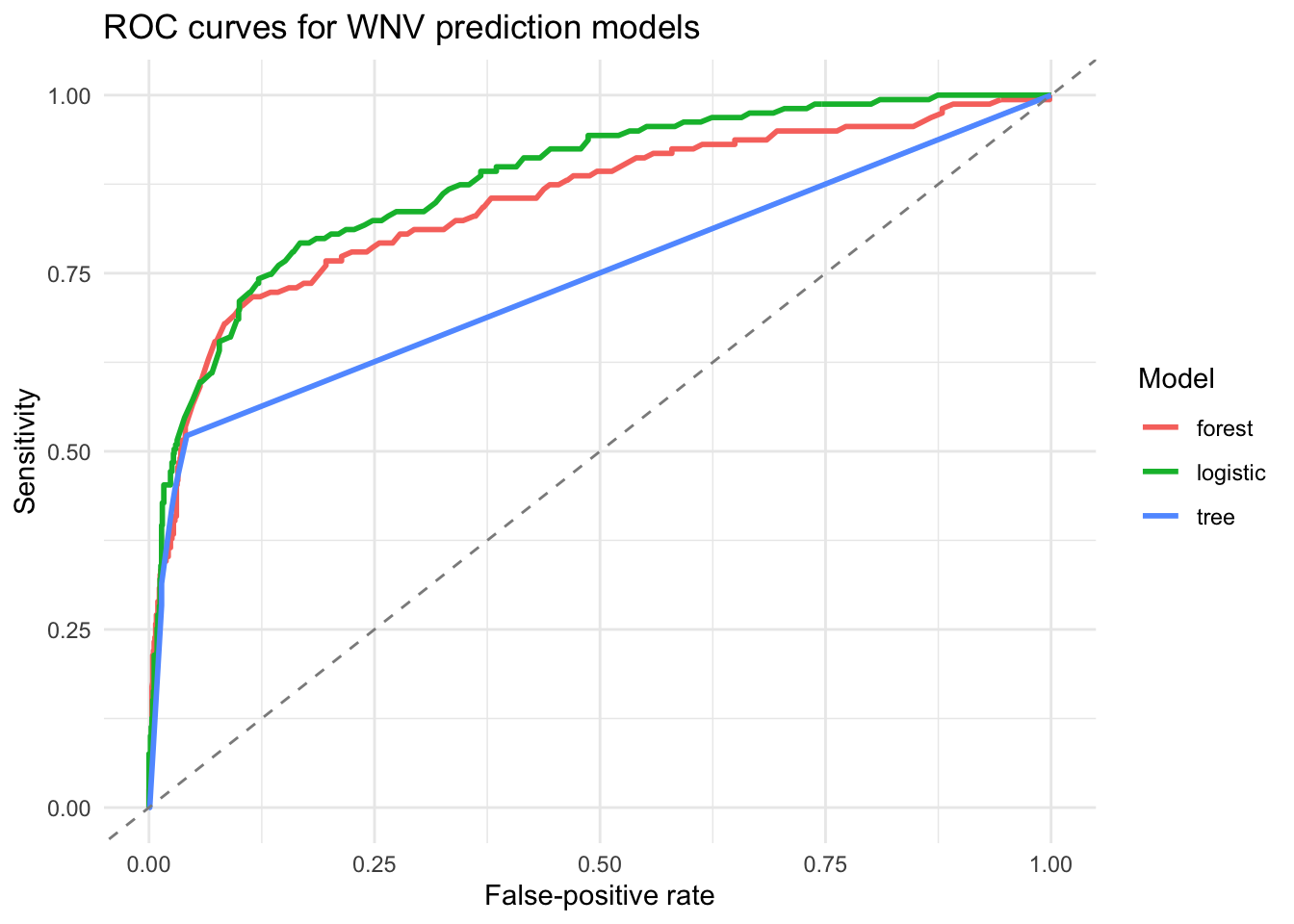

Confusion matrix plot

confusion_data <- rbindlist(lapply(unique(holdout_predictions$model), function(m) {
  pred <- holdout_predictions[model == m]
  pred$response <- ifelse(pred$probability >= 0.5, "yes", "no")
  tab <- table(Actual = pred$truth, Predicted = pred$response)
  data.table(
    model = m,
    truth = rep(c("no", "yes"), each = 2),
    response = rep(c("no", "yes"), times = 2),
    count = as.vector(tab)
  )
}))

ggplot(confusion_data, aes(response, truth, fill = count)) +
  geom_tile(color = "white") +
  geom_text(aes(label = count), fontface = "bold") +
  scale_fill_gradient(low = "#F3E8FF", high = "#6D28D9") +
  facet_wrap(~ model) +
  labs(
    title = "Confusion matrices on the 2025 holdout set",
    x = "Predicted class",
    y = "Observed class",
    fill = "Count"
  ) +
  theme_minimal()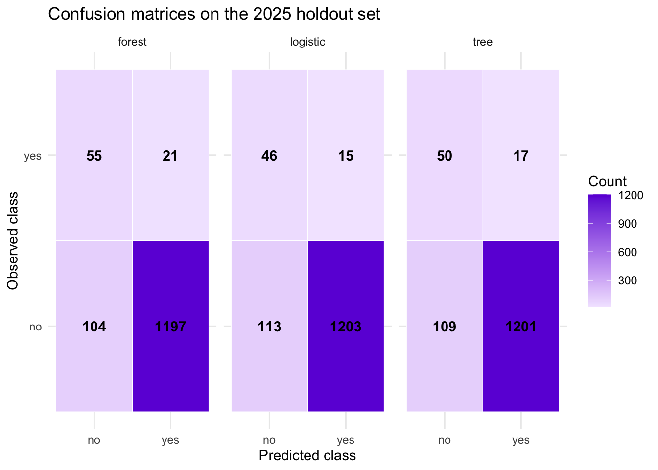

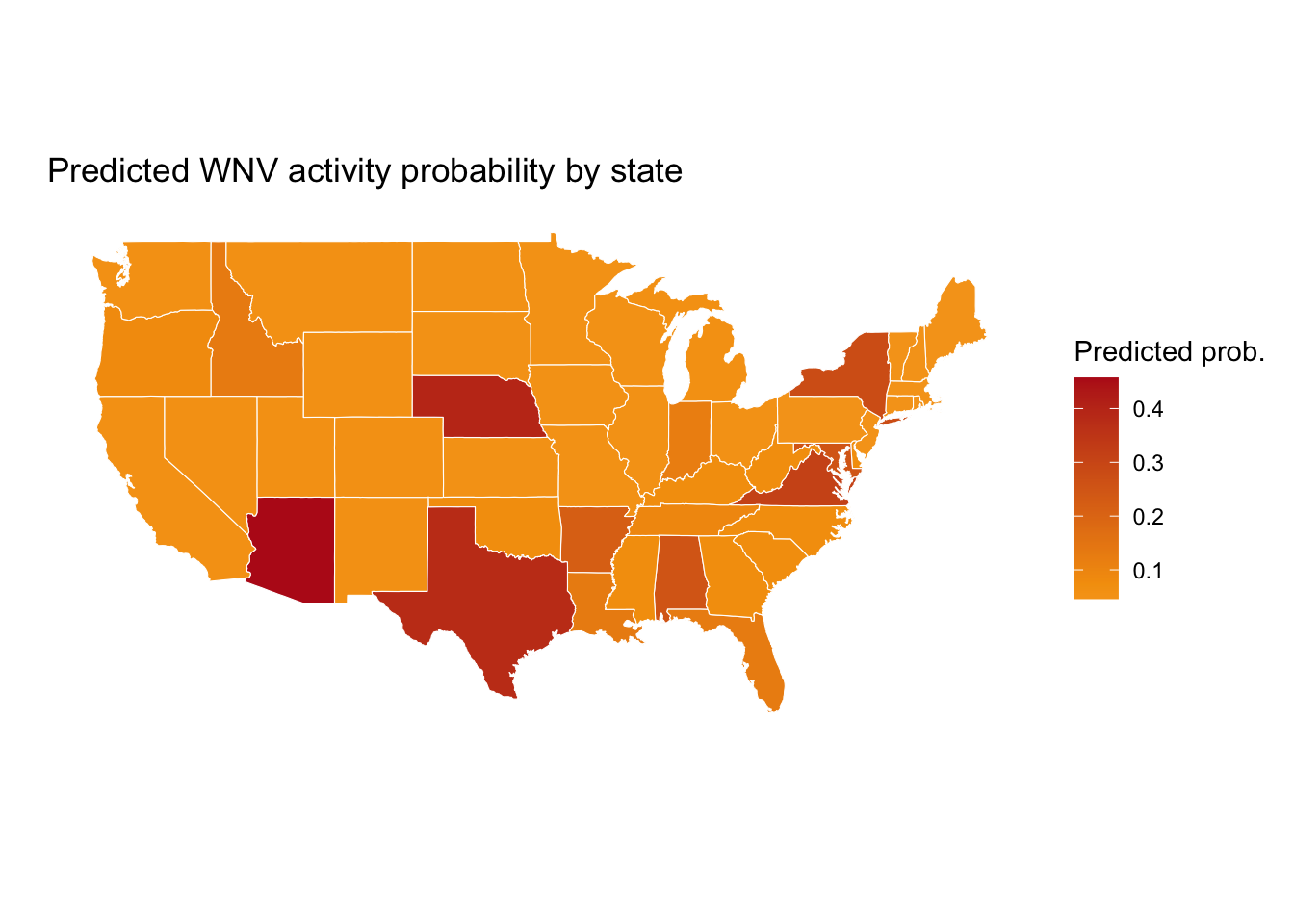
Geographic map of predictions

state_predictions <- holdout_predictions |> 
  group_by(state) |>
  summarise(predicted_probability = mean(probability), .groups = "drop")

state_map <- map_data("state")
state_map <- state_map |>
  rename(state = region) |>
  left_join(
    state_predictions |> mutate(state = tolower(state)),
    by = "state"
  )

ggplot(state_map, aes(long, lat, group = group, fill = predicted_probability)) +
  geom_polygon(color = "white", linewidth = 0.2) +
  coord_map() +
  scale_fill_gradient2(
    low = "#FDE68A",
    mid = "#F59E0B",
    high = "#B91C1C",
    midpoint = median(state_map$predicted_probability, na.rm = TRUE)
  ) +
  labs(
    title = "Predicted WNV activity probability by state",
    x = "",
    y = "",
    fill = "Predicted prob."
  ) +
  theme_minimal() +
  theme(
    panel.grid = element_blank(),
    axis.text = element_blank(),
    axis.ticks = element_blank()
  )

---

11. What the results mean

The point of the workflow is not only to fit a model but to explain how machine learning works in practice.

A typical sequence is:

• Use historical data to learn patterns.
• Choose a model and specify the outcome.
• Train the model on observed labels.
• Predict on unseen data.
• Evaluate the output with appropriate metrics.
• Interpret the model in context.

This is the bridge between the abstract learning cycle and applied epidemiology.

---

12. Final takeaway

The conceptual notebook shows that learning is about using data to update model parameters or structure according to a loss function and an optimization scheme.

The epidemiology workflow shows how the same logic is used in a real decision problem: predict whether WNV activity will be observed in future weeks using information available at the current time.

The same essential pattern appears in both:

data -> model -> predictions -> loss -> update -> repeat -> evaluation

That is the heart of machine learning.